
Project 2
Week 13- Wednesday
In class, we learnt following topics:
1. Convert Dates to Datetime Objects
– ‘pd.to_datetime()’ is used to convert the ‘issued_date’ and ‘expiration_date’ columns in the DataFrame `data` to datetime objects.
– ‘errors=’coerce” is employed to handle any parsing errors, converting problematic entries to NaT (Not a Time).
– ‘pd.to_datetime()’ is used to convert the ‘issued_date’ and ‘expiration_date’ columns in the DataFrame `data` to datetime objects.
– ‘errors=’coerce” is employed to handle any parsing errors, converting problematic entries to NaT (Not a Time).
Code:
data[‘issued_date’] = pd.to_datetime(data[‘issued_date’], errors=’coerce’)
data[‘expiration_date’] = pd.to_datetime(data[‘expiration_date’], errors=’coerce’)
2. Calculate Duration
– The ‘duration’ column is created, representing the number of days between ‘expiration_date’ and ‘issued_date’.
– The ‘duration’ column is created, representing the number of days between ‘expiration_date’ and ‘issued_date’.
Code:
data[‘duration’] = (data[‘expiration_date’] – data[‘issued_date’]).dt.days
3. Visualization – Number of Permits Issued Over Time
– A new column ‘issued_year’ is created, extracting the year from the ‘issued_date’.
– A bar plot (‘sns.countplot()’) is generated using Seaborn to visualize the count of permits issued each year.
– Matplotlib functions are then utilized to add labels, title, and rotate the x-axis ticks for better readability.
– Finally, ‘plt.show()’ displays the resulting bar chart.
Code:
data[‘issued_year’] = data[‘issued_date’].dt.year
plt.figure(figsize=(10, 6))
sns.countplot(data=data, x=’issued_year’)
plt.title(‘Number of Permits Issued Over Time (by Year)’)
plt.xlabel(‘Year’)
plt.ylabel(‘Number of Permits’)
plt.xticks(rotation=45)
plt.tight_layout()
plt.show()
In summary, the whole code transforms date columns, calculates the duration between them, and creates a visualization to show the distribution of permits issued over different years. The Seaborn and Matplotlib libraries are used for data manipulation and visualization.
Project 1
Week 10- Monday
This is Project 2 for MTH 522
Project Title:
Spatial and Demographic Analysis of Police Shootings Related to Police Station Locations in the United States
project 2Week 7- Friday
Hierarchical Clustering
Unlike K-mean clustering Hierarchical clustering starts by assigning all data points as their own cluster. As the name suggests it builds the hierarchy and in the next step, it combines the two nearest data point and merges it together to one cluster.
1. Assign each data point to its own cluster.
2. Find closest pair of cluster using Euclidean distance and merge them in to single cluster.
3. Calculate distance between two nearest clusters and combine until all items are clustered in to a single cluster.
In this technique, you can decide the optimal number of clusters by noticing which vertical lines can be cut by horizontal line without intersecting a cluster and covers the maximum distance.
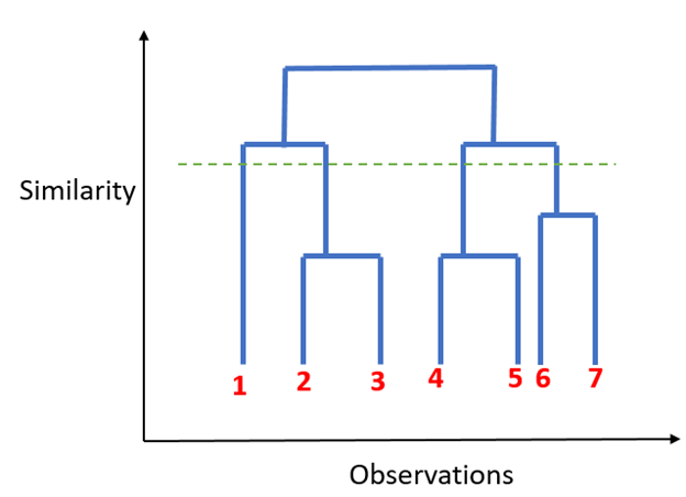
Dendogram
Things to remember when using clustering algorithm:
- Standardizing variables so that all are on the same scale. It is important when calculating distances.
- Treat data for outliers before forming clusters as it can influence the distance between the data points.
Week 7- Monday
Clustering — Unsupervised Learning
What is Clustering?
“Clustering” is the process of grouping similar entities together. The goal of this unsupervised machine learning technique is to find similarities in the data point and group similar data points together.
Why use Clustering?
Grouping similar entities together help profile the attributes of different groups. In other words, this will give us insight into underlying patterns of different groups. There are many applications of grouping unlabeled data, for example, you can identify different groups/segments of customers and market each group in a different way to maximize the revenue.
Another example is grouping documents together which belong to the similar topics etc.
Clustering is also used to reduces the dimensionality of the data when you are dealing with a copious number of variables.
How does Clustering algorithms work?
There are many algorithms developed to implement this technique but for this post, let’s stick the most popular and widely used algorithms in machine learning.
- K-mean Clustering
- Hierarchical Clustering
K-mean Clustering
It starts with K as the input which is how many clusters you want to find. Place K centroids in random locations in your space.
Now, using the Euclidean distance between data points and centroids, assign each data point to the cluster which is close to it.
Recalculate the cluster centers as a mean of data points assigned to it.
Repeat 2 and 3 until no further changes occur.
Now, you might be thinking that how do I decide the value of K in the first step.
One of the methods is called “Elbow” method can be used to decide an optimal number of clusters. Here you would run K-mean clustering on a range of K values and plot the “percentage of variance explained” on the Y-axis and “K” on X-axis.
In the picture below you would notice that as we add more clusters after 3 it doesn’t give much better modeling on the data. The first cluster adds much information, but at some point, the marginal gain will start dropping.
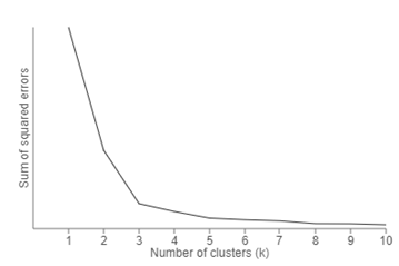
Elbow Method
Week 6- Friday
Logistic regression (classification) – text chapter 4
After watching the video, we have discussed the following terminologies in the class.
- Review of Logistic Regression Concepts:
- Recap of fundamental concepts in logistic regression, a statistical technique used for predicting binary outcomes. It involves understanding the logistic function, odds ratio, decision boundaries, and the process of maximum likelihood estimation.
- Coefficients for Continuous Variables:
- Numeric values assigned to continuous variables in logistic regression. These coefficients represent the change in log-odds for the outcome variable associated with a one-unit change in the continuous predictor.
- Coefficients for Discrete Variables:
- Weights assigned to dummy variables that represent discrete categories in logistic regression. These coefficients indicate how much the log-odds of
the outcome change compared to a chosen reference category.
- Weights assigned to dummy variables that represent discrete categories in logistic regression. These coefficients indicate how much the log-odds of
- Coefficients for Combinations of Variable Types:
- Weights associated with logistic regression models that include a mix of continuous and discrete variables. These coefficients demonstrate the joint influence of different types of variables on the log-odds of the predicted outcome.
Week 6 – Wednesday
This report conducts a thorough examination of demographic elements in incidents of police shootings, utilizing data sourced from the Washington Post Police Shootings Database.
Our primary objective is to enhance our understanding of age distribution, race, mental health status, gender, and other pertinent factors associated with instances of police violence.
Age Distribution:
The analysis of age distribution aims to uncover patterns and disparities, providing insights into the prevalence of police violence across various age brackets.
Mental Illness as a Condition:
We delve into the occurrence of mental illness, underscoring the significance of mental health and advocating for appropriate interventions and support.
Gender:
Through the examination of gender disparities, we contribute to discussions surrounding gender-related aspects of police violence.
Other Factors:
Additional dataset factors such as location and time of day are taken into account to glean insights into the contextual details of these incidents.
This report serves as a valuable asset for policymakers, law enforcement professionals, and advocacy groups dedicated to criminal justice reform. Our insights, rooted in data analysis, aspire to facilitate evidence-based decision-making and address concerns pertaining to police shootings.
Week 6- Monday
My main focus is on analyzing the various variables present in the provided dataset from the Washington Post, particularly emphasizing the examination of their interrelationships. The dataset revolves around fatal police shootings and encompasses two distinct sets of data.
The second dataset specifically furnishes information about law enforcement officers linked to these incidents.
Key variables in this dataset include ID, Name, Type (officers’ roles), States, ORI codes, and Total Shootings. Upon scrutinizing this data, a notable observation is the prevalence of officers associated with local police departments, and the highest recorded number of fatal shootings attributed to a single officer is 129.
In the earlier blog entry, I offered an overview of the first dataset, highlighting its 12 variables.
The primary goal is to investigate potential correlations among these variables. Additionally, I pinpointed crucial features that could establish connections between the two datasets for future analyses.
In the forthcoming blog post, I intend to delve deeper into these variables, further exploring the correlations that can be derived from them.